Kernel Functions

Kernel methods (Shawe-Taylor and Cristianini, 2004) are a powerful class of algorithms for pattern analysis that, exploiting the so called kernel functions, can operate in an implicit high-dimensional feature space without explicitly computing the coordinates of the data in that space. Most of the existing machine learning platforms provide kernel methods that operate only on vectorial data. On the contrary, KeLP has the fundamental advantage that there is no restriction on a specific data structure, and kernels directly operating on vectors, sequences, trees, graphs, or other structured data can be defined.

Furthermore, another appealing characteristic of KeLP is that kernels can be composed and combined in order to create richer similarity metrics in which different information from different Representations can be simultaneously exploited.

As shown in the figure below, KeLP completely supports the composition and combination mechanisms providing three abstractions of the Kernel class:

DirectKernel: in computing the kernel similarity it operates directly on a specific Representation that it automatically extracts from the Examples to be compared. For instance, KeLP implements LinearKernel on Vector representations, and SubTreeKernel (Collins and Duffy, 2001) and PartialTreeKernel (Moschitti, 2006) on TreeRepresentations.
KernelComposition: it enriches the kernel similarity provided by any another kernel. Some KeLP implementations are PolynomialKernel, RBFKernel and NormalizationKernel.
KernelCombination: it combines different kernels in a specific function. Some KeLP implementations are LinearKernelCombination and KernelMultiplication.

Moreover, the class KernelOnPairs models kernels operating on ExamplePairs: all kernels discussed in (Filice et al., 2015) and the PreferenceKernel (Shen and Joshi, 2003) implement this class.

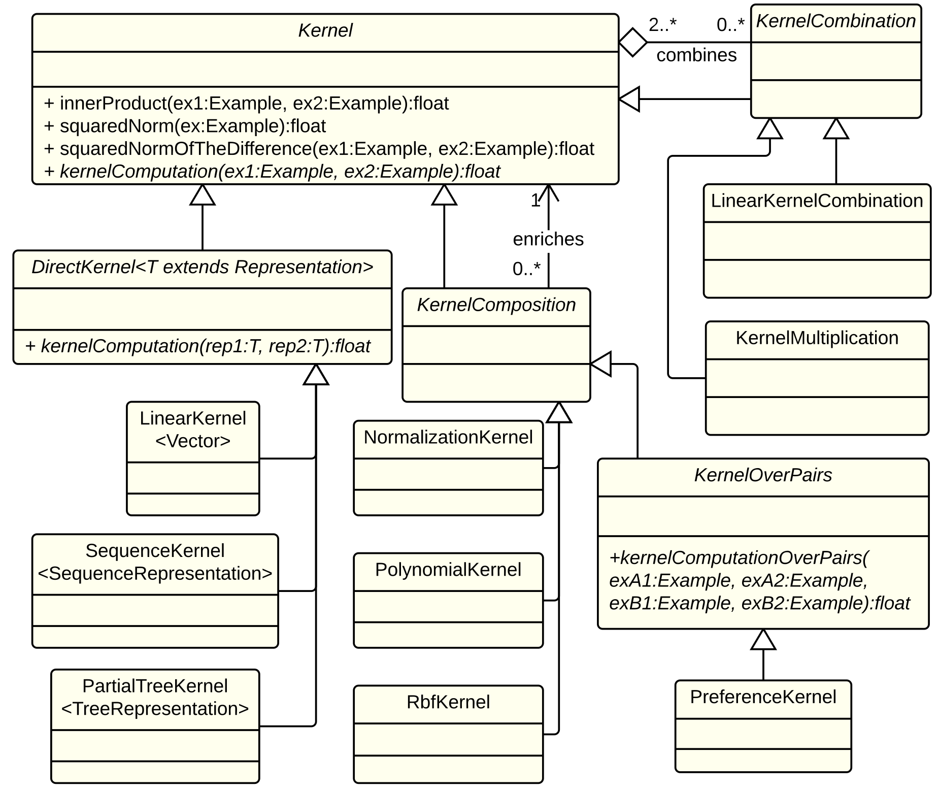
A simplified class diagram of the kernel taxonomy in KeLP.

Existing Kernels

Kernels on Vectors: they are DirectKernels operating on Vector representations (both DenseVector and SparseVector).

LinearKernel: it executes the dot product between two Vector representations.

Kernels on Sequences: they are DirectKernels operating on SequenceRepresentions.

SequenceKernel: it is a convolution kernel between sequences. The algorithm corresponds to the recursive computation presented in (Bunescu and Mooney, 2005).

Kernels on Trees: they are DirectKernels operating on TreeRepresentions.

a) Constituency parse tree for the sentence Federer won against Nadal, b) some subtrees, c) some subset trees, d) some partial trees.

SubTreeKernel: it is a convolution kernel that evaluates the tree fragments shared between two trees. The considered fragments are subtrees, i.e., a node and its complete descendancy. For more details see (Vishwanathan and Smola, 2003).
SubSetTreeKernel: the SubSetTree Kernel, a.k.a. Syntactic Tree Kernel, is a convolution kernel that evaluates the tree fragments shared between two trees. The considered fragments are subset-trees, i.e., a node and its partial descendancy (the descendancy can be incomplete in depth, but no partial productions are allowed; in other words, given a node either all its children or none of them must be considered). For further details see (Collins and Duffy, 2001).
PartialTreeKernel: it is a convolution kernel that evaluates the tree fragments shared between two trees. The considered fragments are partial trees, i.e., a node and its partial descendancy (the descendancy can be incomplete, i.e., a partial production is allowed). For further details see (Moschitti, 2006).
SmoothedPartialTreeKernel: it is a convolution kernel that evaluates the tree fragments shared between two trees (Croce et al., 2011). The considered fragments are partial trees (as for the PartialTreeKernel) whose nodes are identical or similar according to a node similarity function: the contribution of the fragment pairs in the overall kernel thus depends on the number of shared substructures, whose nodes contribute according to such a metrics.
This kernel is very flexible as the adoption of node similarity functions allows the definition of more expressive kernels, such as the Compositionally Smoothed Partial Tree Kernel (Annesi et al, 2014).

Kernels on Graphs: they are DirectKernels operating on DirectedGraphRepresentions.

ShortestPathKernel: it associates a feature to each pair of nodes of one graph. The feature name corresponds to pair of node labels while the value is the length of the shortest path between the nodes in the graph. Further details can be found in (Borgwardt and Kriegel, 2005).
WLSubtreeMapper: it is actually an explicit feature extractor that output vectors containing the features of the Weisfeiler–Lehman Subtree Kernel for Graphs (Shervashidze, 2011). A LinearKernel can be used to exploit the produced vectors.

Kernel Compositions: they are kernels that enriches the computation of another kernel.

PolynomialKernel: it implicitly works in a features space where all the polynomials of the original features are available. As an example, a $2^{nd}$ degree polynomial kernel applied over a linear kernel on vector representations will automatically consider pairs of features in its similarity evaluation. Given a base kernel K, the PolynomialKernel applies the following formula: $poly_K(x,y)=\big ( aK(x,y)+b \big ) ^d$ , where $d, a, b$ are kernel parameters. Common values are $d=2$ , $a=1$ and $b=0$ .
RbfKernel: the Radial Basis Function (RBF) Kernel, a.k.a. Gaussian Kernel, enriches another kernel according to the following formula $RBF_K(x,y) = e^{-\gamma \left \lVert x-y \right \rVert_{\mathcal{H}_K} ^2}$ , where: $\left\lVert a \right\rVert_{\mathcal{H}_K}$ is the norm of $a$ in the kernel space ${\mathcal{H}_K}$ generated by a base kernel $K$ . $\left\lVert x-y \right\rVert_{\mathcal{H}_K} ^2$ can be computed as $\left\lVert x-y \right\rVert_{\mathcal{H}_K} ^2 = \left\lVert x \right\rVert_{\mathcal{H}_K} ^2 + \left\lVert y \right\rVert_{\mathcal{H}_K} ^2 - 2K(x,y) = K(x,x) + K(y,y) - 2K(x,y)$ . This allows to apply the RBF operation to any kernel base kernel K. It depends on a width parameter $\gamma$ which regulates how fast the RbfKernel similarity decays w.r.t. the distance of the input objects in ${\mathcal{H}_K}$ . It can be proven that the Gaussian Kernel produces an infinite dimensional RKHS.
NormalizationKernel: it normalizes another kernel K according to the following formula: $N_{K}(x,y) = \frac{K(x,y)}{\sqrt{K(x,x)K(y,y)}} = \frac{\phi(x)\cdot \phi(y)}{\sqrt{ \left \| \phi(x) \right \|^2 \left \| \phi(y) \right \|^2}} = \frac{\phi(x)}{\left \| \phi(x) \right \|} \cdot \frac{\phi(y)}{\left \| \phi(y) \right \|}$ , where $\phi(\cdot)$ is the implicit projection function operated by the kernel K. The normalization operation corresponds to a dot product in the RKHS of the normalized projections of the input instances. When K is LinearKernel on two vectors, the NormalizationKernel equals to the cosine similarity between the two vectors. The normalization operation is required when the instances to be compared are very different in size, in order to avoid that large instances (for instance long texts) are associated with larger similarities. For instance it is usually applied to tree kernels, in order properly compare trees having very different sizes.

Kernel Combinations: they combine different kernels, allowing the possibility to simultaneously exploit different data representations.

LinearKernelCombination: given a set n of Kernels $K_1, \ldots, K_n$ , it computes the weighted sum of the kernel similarities: $K(x,y)\sum_{i\leq n}c_iK_i(x,y)$ where $c_i$ are the parametrizable weights of the combination.
KernelMultiplication: given a set n of Kernels $K_1, \ldots, K_n$ , it computes the product of the kernel similarities: $K(x, y) = \prod_{i\leq n}K_i(x,y)$ .

Kernels on Pairs: They operate on instances of ExamplePair.

PreferenceKernel: In the learning to rank scenario, the preference kernel (Shen and Joshi, 2003) compares two pairs of ordered objects $p_a = \langle a_1, a_2 \rangle$ and $p_b = \langle b_1, b_2 \rangle$ : $K ( p_a, p_b ) = BK(a_1, b_1) + BK(a_2, b_2) - BK(a_1, b_2) - BK(a_2, b_1)$ , where BK is a generic kernel operating on the elements of the pairs. The underlying idea is to evaluate whether the first pair $\langle a_1, a_2 \rangle$ aligns better to the second pair in its regular order $\langle b_1, b_2 \rangle$ rather than to its inverted order $\langle b_2, b_1 \rangle$ .
UncrossedPairwiseSumKernel: it compares two pairs of ordered objects $p_a = \langle a_1, a_2 \rangle$ and $p_b = \langle b_1, b_2 \rangle$ , summing the contributions of the single element similarities: $K ( p_a, p_b ) = BK(a_1, b_1) + BK(a_2, b_2)$ , where BK is a generic kernel operating on the elements of the pairs. It has been used in learning scenarios where the elements within a pair have different roles, such as text and hypothesis in Recognizing Textual Entailment (Filice et al., 2015), or question and answer in Question Answering (Filice et al., 2016).
UncrossedPairwiseProductKernel: it compares two pairs of ordered objects $p_a = \langle a_1, a_2 \rangle$ and $p_b = \langle b_1, b_2 \rangle$ , multiplying the contributions of the single element similarities: $K ( p_a, p_b ) = BK(a_1, b_1) \cdot BK(a_2, b_2)$ , where BK is a generic kernel operating on the elements of the pairs. As for the UncrossedPairwiseSumKernel, it has been used in learning scenarios where the elements within a pair have different roles, such as text and hypothesis in Recognizing Textual Entailment (Filice et al., 2015), or question and answer in Question Answering (Filice et al., 2016). The product operation inherently applies a sort of logic and between the $BK(a_1, b_1)$ and $BK(a_2, b_2)$ .
PairwiseSumKernel: it compares two pairs of objects $p_a = \langle a_1, a_2 \rangle$ and $p_b = \langle b_1, b_2 \rangle$ , summing the contributions of all pairwise similarities between the single elements: $K ( p_a, p_b ) = BK(a_1, b_1) + BK(a_2, b_2) + BK(a_1, b_2) + BK(a_2, b_1)$ , where BK is a generic kernel operating on the elements of the pairs. It has been used in symmetric tasks, such as Paraphrase Identification, where the elements within a pair are interchangeable (Filice et al., 2015).
PairwiseProductKernel: it compares two pairs of objects $p_a = \langle a_1, a_2 \rangle$ and $p_b = \langle b_1, b_2 \rangle$ , summing the contributions of the two possible pairwise alignments: $K ( p_a, p_b ) = BK(a_1, b_1) \cdot BK(a_2, b_2) + BK(a_1, b_2) \cdot BK(a_2, b_1)$ , where BK is a generic kernel operating on the elements of the pairs. It has been used in symmetric tasks, such as Paraphrase Identification, where the elements within a pair are interchangeable (Filice et al., 2015).
BestPairwiseAlignmentKernel: it compares two pairs of objects $p_a = \langle a_1, a_2 \rangle$ and $p_b = \langle b_1, b_2 \rangle$ , evaluating the best pairwise alignment: $K( p_a, p_b ) = softmax \Big ( BK(a_1,b_1) \cdot BK(a_2, b_2), BK(a_1,b_2) \cdot BK(a_2,b_1) \Big )$ , where BK is a generic kernel operating on the elements of the pairs, and softmax is a function put in place of the max operation, which would cause K not to be a valid kernel function (i.e., the resulting Gram matrix can violate the Mercer’s conditions). In particular, $softmax$(x_1,x_2)= \frac{1}{c} \log(\exp(c x_1) + \exp(c x_2)$ (c=100 is accurate enough). The BestPairwiseAlignmentKernel has been used in symmetric tasks, such as Paraphrase Identification (Filice et al., 2015), where the elements within a pair are interchangeable.

References

Paolo Annesi, Danilo Croce, and Roberto Basili. Semantic compositionality in tree kernels. In Proceedings of the 23rd ACM International Conference on Conference on In- formation and Knowledge Management, CIKM ’14, pages 1029–1038, New York, NY, USA, 2014. ACM.

K. M. Borgwardt and H.–P. Kriegel. Shortest–Path Kernels on Graphs. in Proceedings of the Fifth IEEE International Conference on Data Mining, 2005, pp. 74–81.

Razvan C. Bunescu and Raymond J. Mooney. Subsequence kernels for relation extraction. 2005. In NIPS.

Michael Collins and Nigel Duffy. Convolution kernels for natural language. In Proceedings of the 14th Conference on Neural Information Processing Systems, 2001.

Danilo Croce, Alessandro Moschitti, and Roberto Basili. Structured lexical similarity via convolution kernels on dependency trees. In Proceedings of EMNLP, Edinburgh, Scotland, UK., 2011.

Simone Filice, Giovanni Da San Martino and Alessandro Moschitti. Relational Information for Learning from Structured Text Pairs. In Proceedings of the 53^rd Annual Meeting of the Association for Computational Linguistics, ACL 2015.

Simone Filice, Danilo Croce, Alessandro Moschitti and Roberto Basili. KeLP at SemEval-2016 Task 3: Learning Semantic Relations between Questions and Answers. In Proceedings of the 10th International Workshop on Semantic Evaluation (SemEval 2016), Association for Computational Linguistics. (Best system @ SemEval-2016 task 3)

Alessandro Moschitti. Efficient convolution kernels for dependency and constituent syntactic trees. In ECML, Berlin, Germany, September 2006.

Libin Shen and Aravind K. Joshi. An svm based voting algorithm with application to parse reranking. In In Proc. of CoNLL 2003, pages 9–16, 2003

John Shawe-Taylor and Nello Cristianini. Kernel Methods for Pattern Analysis. Cambridge University Press, New York, NY, USA, 2004. ISBN 0521813972.

N. Shervashidze, Weisfeiler–lehman graph kernels, JMLR, vol. 12, pp. 2539–2561, 2011

S.V.N. Vishwanathan and A.J. Smola. Fast kernels on strings and trees. In Proceedings of Neural Information Processing Systems (NIPS), 2003.

Fabio massimo Zanzotto, Marco Pennacchiotti, and Alessandro Moschitti. A machine learning approach to textual entailment recognition. Nat. Lang. Eng., 15(4): 551–582, October 2009. ISSN 1351-3249.